Scale your dot product in attentions

Seq2Seq models were a common approach for translation tasks before transformers. But this had a “bottleneck” problem due to it’s fixed length hidden state vector that led to poor compression of the source sequence information and difficulty in handling long sequences. Attention was introduced to reduce the burden on the final hidden state and to query specific source information based on what is necessary for the decoder to predict the next token.

Note: This article analyses the importance of scaling with respect to Luong’s attention but this is applicable to modern transformers as well.

> If you know dot product attention in language models, Skip to the scaling problem section

Dot product in attention

Luong et. al improved the additive attention technique introduced earlier with several modifications like

Pure language modelling in decoder - by moving attention block outside the decoder. The decoder state can now purely do its language modelling without the influence of encoder’s representation.
Input feeding - Makes the attention stateful across time and avoids focusing on the same source token multiple times.
Dot product score function - Instead of adding the encoder and decoder hidden states, this used dot product to calculate the attention scores for each source token.

Model setup

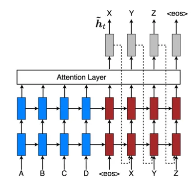
Here’s how it works

The encoder encodes the source sequence and produces the final hidden state which is used to initialise the decoder
The decoder produces the current hidden state based on the last predicted token or <bos> token as the input.
Before predicting the next output token, the decoder state and all the encoder states are used by the attention layer to create the context. This attended context is used to predict the output token

Luong Architecture

Attention layer

Attention allows the decoder to selectively focus on the most relevant parts of the input sequence at each time step. It computes weights over encoder states and generates a context vector, helping the model capture long range dependencies and generate more accurate and aligned output tokens using this weighted context.

Let $h_{d}^t$ be the decoder hidden state at time step $t$ and $\{h_{e}^0 \dots h_{e}^{T_{x}}\}$ be all the encoder hidden states at each time step till $T_{x}$ , the length of the source sequence.

Generally, the attention is formulated in this manner. There is a score function which computes a score for each encoder state depending on the current decoder state to indicate which token to attend to from the source. The scores are then normalised using the softmax function to get the “attention weights”,

\begin{align*} a_{t}^i &= \text{softmax}(\text{score}_{i}) \\ &= \frac{\exp(\text{score}(h_{d}^t, h_{e}^i))}{ \sum_{j} \exp(\text{score}(h_{d}^t, h_{e}^j))} \end{align*}

The context vector is computed as weighted sum of all encoder states,

\begin{align*} c_{t} &= \sum_{j=1}^{T_{x}} a_{t}^{j} h_{e}^j \end{align*}

Finally the output token is predicted by concatenating the context vector and decoder state by

\begin{align*} \tilde{y}_{t} &= \tanh(W_{c}[c_{t};h_{d}^t]) \end{align*}

The score function that we focus on in this article is the dot product score

\begin{align*} \text{score}_{i}(h_{d}^t, h_{e}^i) &= {h_{d}^t}^\top h_{e}^i ; \quad i = 1 \dots T_{x} \end{align*}

Why dot product is nice?

A dot product between two vectors represents the magnitude of the similarity in directions they point to. These are the values it can take

positive - when the vectors point in the similar direction
negative - when they point in opposite directions
zero - when they are perpendicular

Since we are working with attention, attention’s objective to find similar tokens in source sequence to the decoder token perfectly matches the property of the dot product. With dot product as the score function, tokens with similar meanings point in the same direction in this vector space resulting in higher score and vice versa.

Assumption: It is important to note that using dot product as score function assumes that the encoder and decoder hidden states lie in the same vector space. This may not be true for all problems. Unlike in Luong attention, the query and key vectors in transformers are linearly transformed and brought to the same vector space before applying the dot product.

Naive implementation of dot product attention

I implemented this attention for a German to English translation task.

python

class DotProductAttention(nn.Module):
    def __init__(self):
        super().__init__()

    def forward(self, decoder_hidden_states, encoder_outputs, mask): # decoder_hidden_states: (num_layers, B, 2 * hidden_dim), encoder_outputs: (B, T, 2 * hidden_dim) bidirectional LSTM
        # use the last hidden state of the multi-layer LSTM decoder as the query
        query = decoder_hidden_states[-1] # (B, 2 * hidden_dim)
        query = query.unsqueeze(2) # (B, 2 * hidden_dim, 1)

        energy = encoder_outputs @ query # (B, T, 1)
        energy = energy.squeeze(2) # (B, T)
        energy = energy.masked_fill(mask, -1e9)
		
        attention_weights = F.softmax(energy, dim=1) # (B, T)
        return attention_weights

There was no improvement in the performance compared to the additive attention and to add to the surprise, the attention weight distribution was not diagonal as I expected 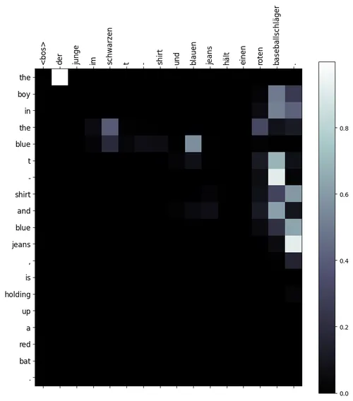Attention weights of unscaled dot product The attention weights were clumped together with the last 2 source tokens. This shows that the attention was basically non-existent and the model behaved like an attention-less sentence embedding model.

Debugging the attention collapse

I had to come up with few hypotheses for this “attention collapse”.

Since the decoder is initialised with the last encoder state, could the dot product score align better with last states?
Last few encoder states contain the complete information about the source sequence unlike the earlier ones. Does the information density make it work well with dot product?
Could the higher norm of last encoder states result in higher dot product?

To find out, I plotted some statistics of the scores for few sequence pairs of the trained model. 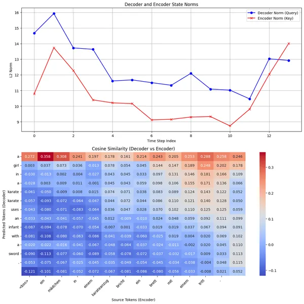Norm and cosine similarity of unscaled attention The norms of the encoder and decoder states is floating around 14 while the cosine similarity plot shows a similar picture as the attention weights.

Looking at the properties of the inputs didn’t give any insights about the attention collapse. So I analysed the statistics of the scores(or energy as sometimes called) once they are multiplied. 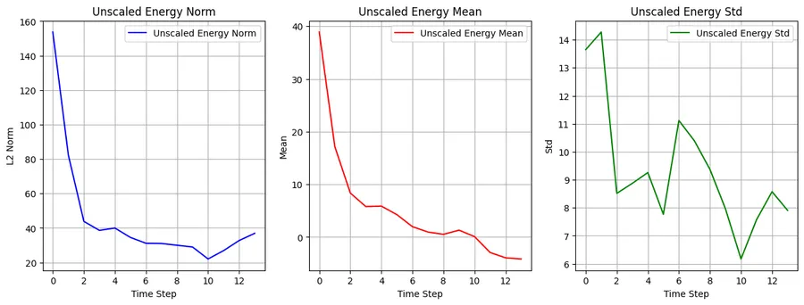Statistics of the unnormalised scores This gives a better idea about what might be happening. The norms of the score ranged from $(20, 160)$ , mean from $(-5, 40)$ and the standard deviation from $(6, 14)$ .

It turns out, there was no problem with the encoder and decoder states and how they were initialised although it still contributed to the anomaly. The anomaly was happening in the scores that were passed to the softmax normalisation due to such a wide range of values.

Limits of Softmax magic

Softmax function just like in most cases, is used in the attention layer to normalise the attention scores of arbitrary range into a probability distribution. This normalised values from $(0,1)$ can be used to create the context as a weighted sum of encoder states.

\begin{align*} \text{softmax}(z_{i}) &= \frac{e^{z_{i}}}{\sum_{j=1}^K e^{z_{j}}} \end{align*}

Taking an “arbitrary range” of numbers to a neat $(0,1)$ distribution seems almost magical. Let’s test this magic and push it to the limits.

python

import numpy as np
import matplotlib.pyplot as plt

def softmax(x):
    x = x - np.max(x)  # numerical stability
    e = np.exp(x)
    return e / np.sum(e)

# Base logits (dot products before scaling)
base_logits = np.array([1.0, 0.8, 0.3, -0.2])

scales = np.linspace(0.1, 50, 400)
max_probs = []
entropies = []

for s in scales:
    p = softmax(base_logits * s)
    max_probs.append(np.max(p))
    entropies.append(-np.sum(p * np.log(p + 1e-12)))

plt.figure()
plt.plot(scales, max_probs, label="Max softmax probability")
plt.plot(scales, entropies, label="Entropy")
plt.xlabel("Logit scale")
plt.ylabel("Value")
plt.legend()
plt.title("Softmax collapse with increasing logit scale")
plt.show()

Softmax function collapse

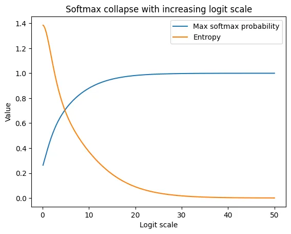
The “Blue” curve represents the maximum probability of a single element after the softmax normalisation as the scale of the vectors increase. As the scale increase beyond 5, most of the area is covered by a single element’s probability and beyond 10 it acts as a one-hot vector where only one element has the probability of 1.0 and 0.0 for the rest. The “Orange” curve shows the entropy of the probability distribution which drastically reduces to 0.0 around the 10 to 15 range. This will act as a useful guide when I use softmax next time where multiplication of large numbers might be involved.

Rule of Thumb: Keep the norm below 5.0 and variance around 1.0 before applying softmax

I plotted the same graph for my attention scores to verify this applies to my model as well. I created random vectors from the norm, mean and deviation from the results above. This confirms the behaviour that we observed in the attention weights heatmap indicating the attention collapse.

Scaled dot product attention implementation

Let’s scale the dot product to reduce the norm by a constant factor of $d_{k}$ , the dimension of the query vector(or encoder state since both of same dimension)

python

class ScaledDotProductAttention(nn.Module):
    def __init__(self):
        super().__init__()

    def forward(
        self, decoder_hidden_states, encoder_outputs, mask
    ):  # decoder_hidden_states: (num_layers, B, 2 * hidden_dim), encoder_outputs: (B, T, 2 * hidden_dim) bidirectional LSTM
        query = decoder_hidden_states[-1]  # (B, 2 * hidden_dim)
        query = query.unsqueeze(2)  # (B, 2 * hidden_dim, 1)

        energy = encoder_outputs @ query  # (B, T, 1)
        energy = energy.squeeze(2)  # (B, T)

        scale = 1.0 / (encoder_outputs.size(-1) ** 0.5)
        energy = energy * scale # <-- scaling happens here
        energy = energy.masked_fill(mask, -1e9)
		
        attention_weights = F.softmax(energy, dim=1)  # (B, T)
        return attention_weights

This improved the BLEU score significantly and the attention weights are distributed as expected 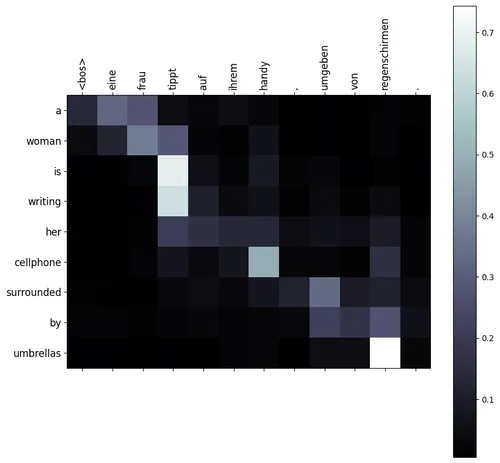Scaled attention weights Finally, the scaled score statistics also shows a much nicer behaviour Scaled attention statistics

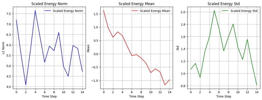
Why scale by $\sqrt{ d_{k} }$ ?

We expect the mean and variance of the encoder and decoder states to be 0.0 and 1.0 respectively because the LSTM or similar RNN model computes the hidden state using $\tanh$ activation. As it can be seen from the scaled standard deviation plot, we want to keep the variance of the score to 1.0 to help the softmax function work optimally. For input variables with such statistical properties it can be proved that the variance of dot product is $d_{k}$ as given in this nice proof.

Thus we divide the scores by its standard deviation which is $\sqrt{ d_{k} }$ to get the desired properties for our unnormalized scores. The observations neatly fit this theory too.

Need for this article

In hind sight, it feels like a minor lack of understanding about the limits of softmax function that led to this analysis but surprisingly scaling the dot product was not mentioned in the original paper and most popular implementations of dot product attention didn’t perform scaling to mitigate this issue.

In Attention is all you need, they have given their reasoning for doing this,

While for small values of $d_{k}$ the two mechanisms perform similarly, additive attention outperforms dot product attention without scaling for larger values of $d_{k}$ . We suspect that for large values of $d_{k}$ , the dot products grow large in magnitude, pushing the softmax function into regions where it has extremely small gradients 4. To counteract this effect, we scale the dot products by $\frac{1}{\sqrt{ d_{k} }}$

I had a fun experience analysing this unexpected result and figuring out the reason behind this behaviour and update my understanding about softmax function and large values in general about neural networks.

This notebook contains the complete model training of the German to English translation using unscaled and scaled dot product attentions.

Remember the assumption we made while using dot product for attention, this notebook analyses a more general dot product attention and compares the results to test this assumption.

Scale your dot product in attentions

Dot product in attention

Model setup

Attention layer

Why dot product is nice?

Naive implementation of dot product attention

Debugging the attention collapse

Limits of Softmax magic

Scaled dot product attention implementation

Why scale by dk\sqrt{ d_{k} }dk​​?

Need for this article

References

Why scale by $\sqrt{ d_{k} }$ ?